Lesson in Development

Analysis using Data Cruncher

So far we have explored running DGE analysis using a public app based on DESeq2. In the second approach, we will set up an interactive analysis on an instance running the RStudio computational environment. We will run a DGE workflow using an analysis script to generate reports and plots.

DGE Tools

While there are other established tools to perform DGE analysis including DESeq2, EdgeR and Limma-Voom, we will be using DESeq2 in our script to allow you to compare the output between the two approaches.

Step 1: Starting Data Cruncher

• Click the Interactive Analysis tab located on the right hand corner below your account settings menu.
• Select Open in the Data Cruncher panel.
• Click on the Create your first analysis which appears the first time your are setting up.
• In the popup box, select RStudio for Environment. Provide an analysis name in the box. Here, Cancer_DGE was used to title the analysis. Click Next when done.
• In the Compute requirements tab, we will use the default instance type (c5.2xlarge, $0.49/hr). We increase the Suspend time, which is the period of inactivity after which the instance is stopped automatically and the analysis is saved, from 30 to 60 minutes.
• Click Start the analysis. This prompts the initialization of the analysis which involves set up of the instance and preparation of the analysis environment.

Instance Types

You can find details on all available US instances from Amazon Web Services (AWS) on Cavatica's Platform Documentation.

Step 2: Navigating analysis editor and load script

After the instance is initialized, you will be automatically directed to the analysis editor which in this case is the RStudio interface.

RStudio IDE

Read more about the different panes and options of the RStudio interface, the integrated development environment (IDE) for the R programing language.

Directory structure

The editor is associated with a directory structure to help you navigate the working space. You can access it via the Files/Packages/Plots/Help/Viewer pane on the bottom right hand corner of RStudio.

/sbgenomics
|–– output-files
|–– project-files
|–– projects
|–– workspace

Important

The project-files directory which contains all the input files is a read only file system while you have read-write permissions for the workspace and output-files directories.

• workspace is the default working directory for the analysis. You can use the RStudio Upload option to get files from your local computer to the workspace.
• output-files can be used as the directory to save all the outputs from your analysis. If not specified, the files are saved to workspace.
• project-files is the directory containing all the input files from the current project. Because it is a read only file system, no changes can be made to these files via the editor interface.

Session outputs

The generated output and environment files from an active session are saved when the analysis is stopped by clicking Stop located on the right hand top corner. You can access the session files via the Files tab in your project folder.

The Data Cruncher comes with a set of libraries that are pre-installed. These vary depending on the environment you chose during setup. We chose the default environment for RStudio SB Bioinformatics - R 4.0 which is loaded with set of CRAN and Bioconductor libraries.

Installing additional libraries

Although the output files, the environment, and history of the session are saved upon stopping the analysis editor, any installed libraries are only good for the session and must be re-installed for every restart of the instance.

Step 3: Run analysis script

Network settings

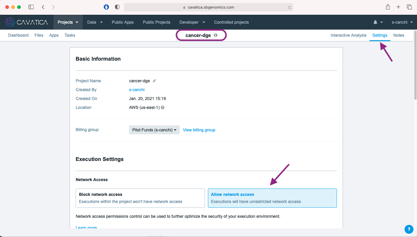
To enable download of packages included in the analysis scripts via internet, it is important to ensure the network access is set to On. Click on Settings within your project folder and select Allow network access box.

You will need to download an analysis script for this step. We have provided you with the option to download two versions of the analysis script based on your choice of execution in RStudio. Click on your preferred option and save the file:

(a) version to execute automatically using Source
(b) version to execute the code in chunks using the Run option.

The (b) version of the script is run manually and contains some additional packages and lines of code to allow for interactive exploration of the data prior to analysis. The DGE analysis and all the generated output are otherwise identical between the two versions.

Upload the script file to the workspace directory. View the upload steps in the vidlet. Briefly:

• Click on the Upload option in the Files/Packages/Plots/Help/Viewer pane.
• Click Choose File to select the file from your local computer.
• Once uploaded, click on the script file name to open it in the script editor pane (top left hand corner).
• To execute go to Step 3a if you chose the (a) version or Step 3b if you chose (b).

Phenotype File Name

For the scripts to run error-free ensure that the name of the phenotype CSV file is "phenotype_filtered.csv". Otherwise, update the R script file if your CSV file has a different name before execution.

Step 3a: Execute using Source version

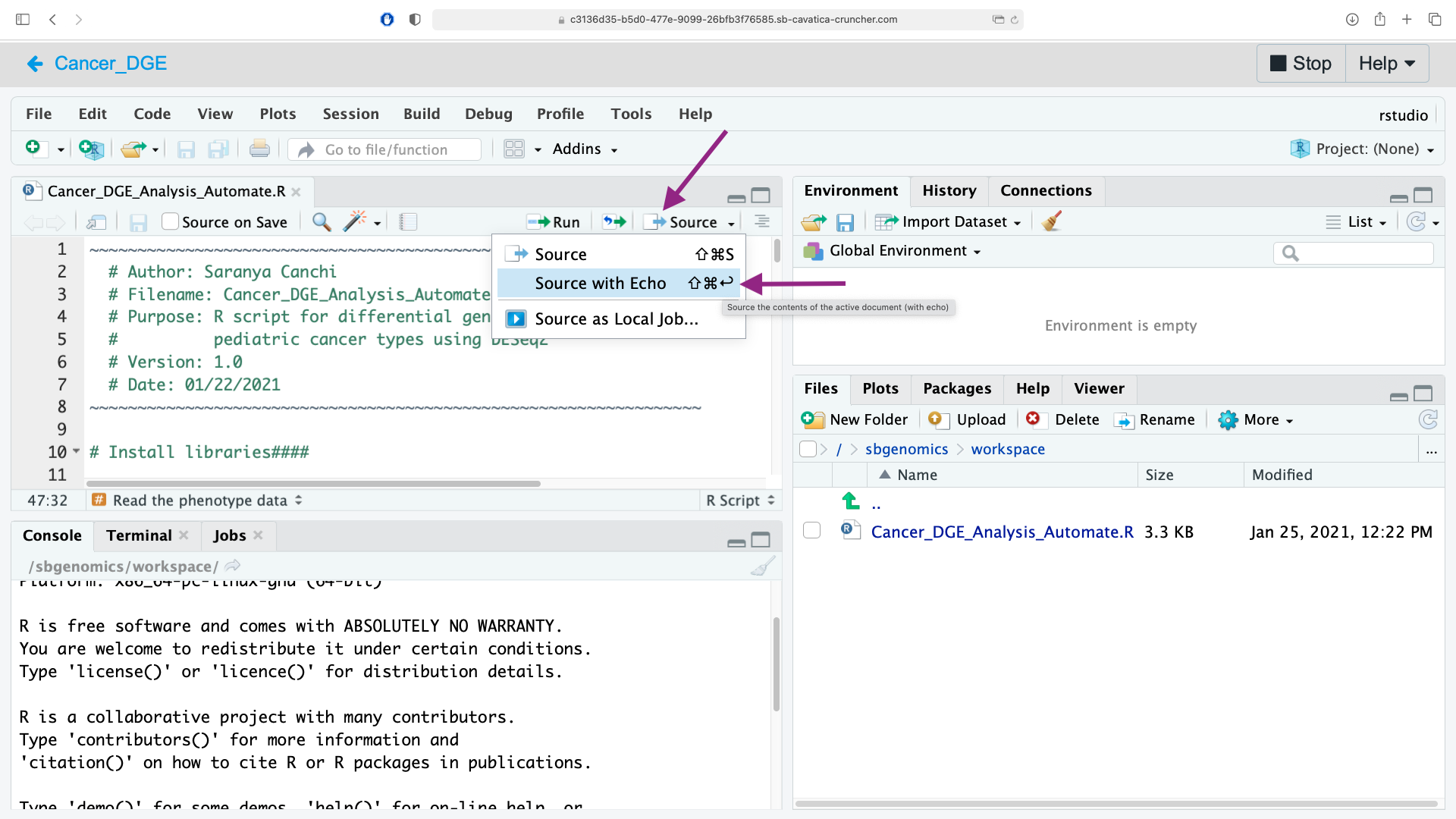
To get started, click on the down arrow next to Source and click Source with Echo. This will print the comments as the code is executed.

This process will take about 15-20 minutes. Once completed, you will get a popup window asking to try to open the html report. Click Try Again to open a new tab for the report.

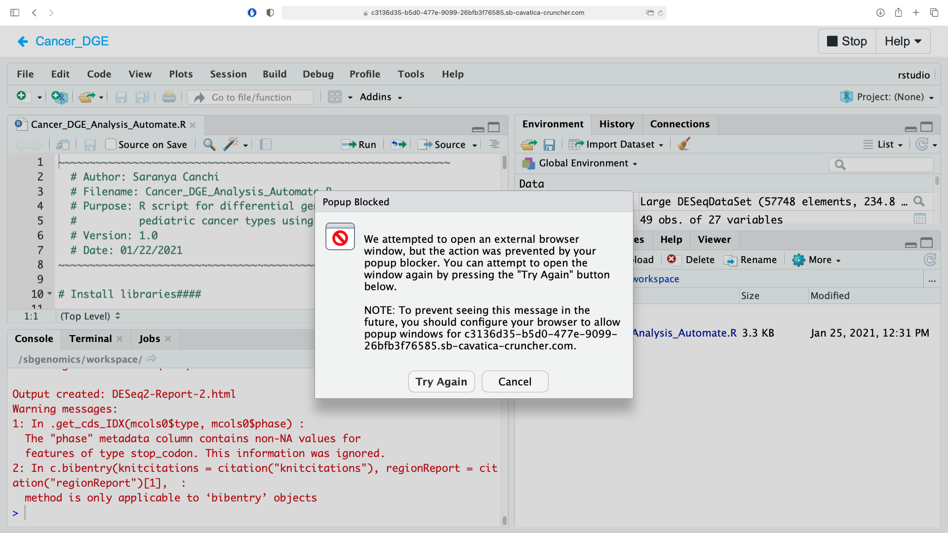
Alternatively, you can click Cancel in the popup window and subsequently click Stop to view the files in your project folder.

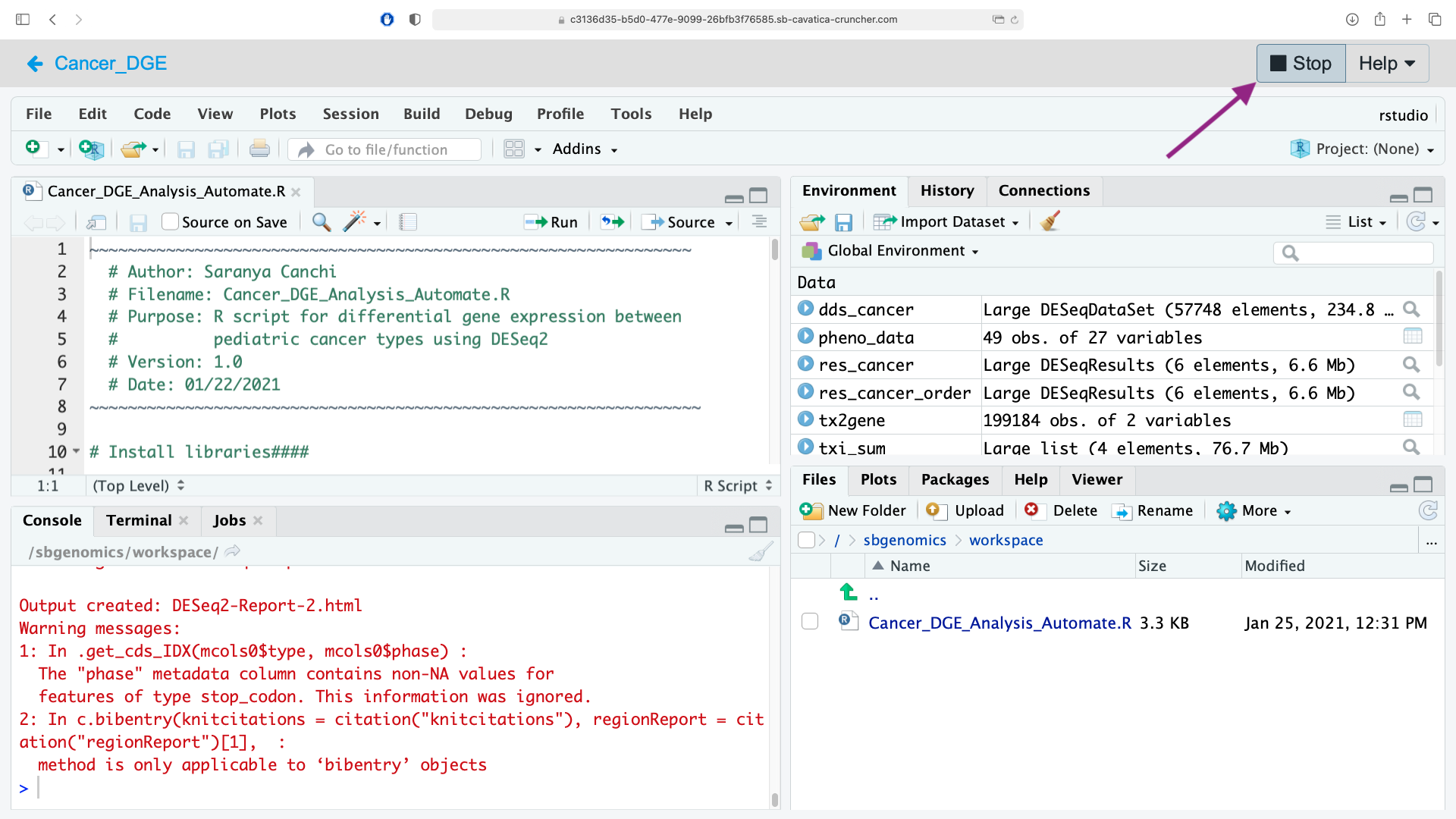
For costs and time comparison between the two approaches, we use the automated version with the option to view the output files in the project folder which took 25 minutes to run and cost $0.2. You are now ready to view your output. Go to Step 4.

Step 3b: Execute using Run version

You can also execute the code by selecting a line or multiple lines of code and clicking the Run option or using Ctrl+Enter keys. This allows you greater flexibility to explore and understand the outputs of each line of code.

The first step is installing the packages necessary for DGE analysis and this takes approximately 17 minutes. Highlight the package install section as shown in the image below and click Run.

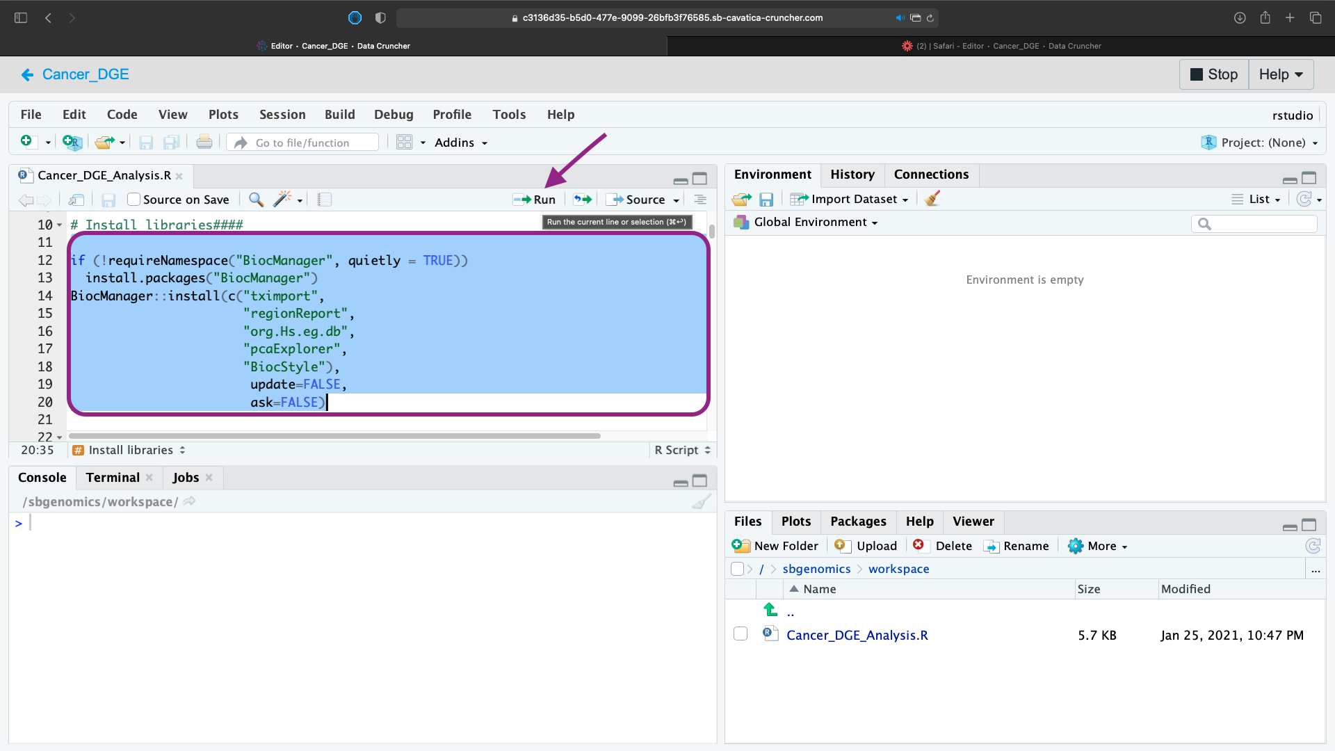
This version includes the Bioconductor package pcaExplorer, which provides interactive visualization of RNA-Seq datasets based on Principal Components Analysis.

After running lines 1-99 of the R script, you should see an interactive output from the pcaExplorer() command. Watch the video below to learn how to use pcaExplorer for the filtered cancer dataset.

When you are finished running the R script, click Stop to view the output files in your Cavatica project folder.

Login Timeout

It is possible to be logged out of Cavatica despite having an active RStudio session. You will be unable to stop the analysis from within the editor using Stop if that occurs.

• Login to Cavatica in a new tab or window.
• Navigate to the data cruncher session via either the Interactive Analysis tab or using the ANALYSES pane in your project home page.

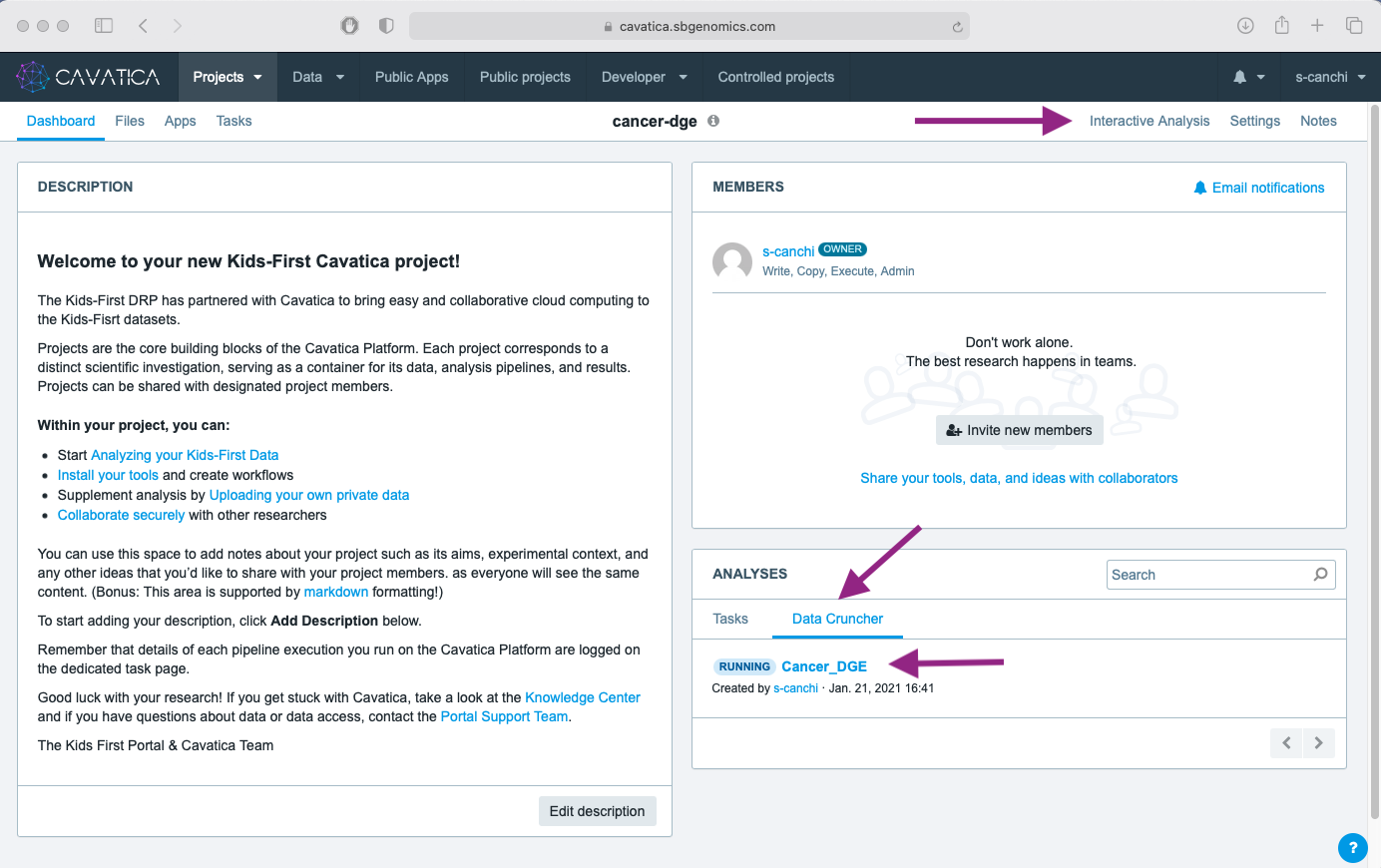
• Click Stop on the session page.

Step 4: View output files

All the session files and the generated outputs are saved after the analysis is stopped and are accessible on the session page.

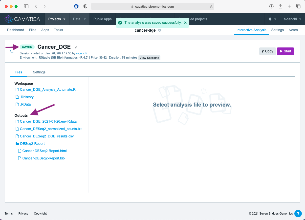
The tag for the session changes from RUNNING to SAVED. Similar to the DESeq2 app, four output files are generated:

• Cancer_DESeq2_DGE_results.csv contains the ordered table of gene level statistics generated using the results() function in DESeq2 package.
• Cancer_DESeq2_normalized_counts.txt contains counts normalized using the estimated sample-specific normalization factors.
• DESeq2-Report folder which contains the HTML report generated using regionReport. The report contains all the visualizations along with the associated code from the DESeq2 vignette.
• Cancer_DGE_{Date}.env.RData is the R workspace image that includes all the objects and variables generated from the code. The .RData listed under Workspace is saved by default by the Data Cruncher.

Output Differences

Although the DGE results are the same between the two analysis approaches, there are some differences between the two html reports since they are not the exact same code. The MA plots generated using Data Cruncher use blue to signify significant genes and the counts plot uses points instead of bars.

All the files are clickable for preview on Cavatica. You can either download individual files by clicking on the file name or follow the steps to tag and download the files listed in the Analysis with DESeq2 Public App lesson.

Conclusion

This concludes the RNA-Seq on Cavatica tutorial. We hope that you found the tutorial helpful and will continue to use cloud computing for your analysis!

Key Points

• The Kids First Portal is the go-to resource for pediatric cancer & structural birth defects datasets.
• Examine data and run analyses using Cavatica, the cloud based analysis platform integrated into Kids First Portal.
• You can filter, view, and download data from Cavatica.
• Upload data to Cavatica from multiple sources including your local machine.
• You can search, copy, and modify a public app on Cavatica.
• Setup and successful run of the DESeq2 app by choosing appropriate inputs.
• Setup a virtual computational environment running RStudio and analyze by executing code from a script.

---

Last update: December 10, 2021