Wrangle Data
Data wrangling is the process of tidying and transforming data to make it more appropriate and valuable for a variety of downstream purposes such as analytics. The goal of data wrangling is to assure quality and useful data. Data analysts typically spend the majority of their time in the process of data wrangling compared to the actual analysis of the data.
Tidying your data means storing it in a consistent form. When your
data is tidy, each column is a variable, and each row is an observation.
Tidy data is important because the consistent structure lets you focus
your struggle on questions about the data, not fighting to get the data
into the right form for different functions. Some tidying functions
include pivot_longer(), pivot_wider(), separate(), unite(),
drop_na(), replace_na(). The lubridate package has a number of
functions for tidying dates. You may also use mutate() function to
convert objects from, say, characters or integers to factors or rename
observations and variables.
Transforming your data includes narrowing in on observations of
interest (like all people in one city, or all data from the last year),
creating new variables that are functions of existing variables (like
computing speed from distance and time), and calculating a set of
summary statistics (like counts or means). Summary functions such as
summarize() and count() to create new tables with statistics. Before
summarizing or counting a whole data frame, you can use group_by() to
group variables. You can use filter() and select() to isolate
specific rows or columns, respectively. If you want to sort columns,
arrange() and arrange(desc()) are two functions to familiarize
yourself with.
Combining tables can be accomplished in one of two ways. If all the
columns or all the rows have all the same names, you can use rbind()
or cbind(), respectively, to join the data frames. If however, each
data frame have a column (or multiple columns) that contain unique
identifiers, then you can use the family of join functions
(inner_join(), outter_join(), left_join(), and right_join())
For each downstream analysis, you will likely use a series of tidying
and transforming steps in various order to get your data in the
appropriate format. Instead of creating dozens of intermediate files
after each step, we will use the %>% operator to “pipe” the output of
one function to the input of the other.
Instead of going into each function or each process in detail in isolation, let’s start with some typical research questions and then piece together R functions to get the desired information.
filter()
Filter is done in a few different ways depending on the type of
variable. You can use > and less < to filter greater or less than a
number. == and != are used to filter by characters or factors that
match or do not match a specific pattern. %in% c() is used to filter
by things in a list. Let’s filter by adjusted p-value. You can use |
and & to mean “or” or “and”
To explore filtering data, let’s answer the following question: What are the approved names and symbols of the differentially expressed genes (DEGs) in the heart tissue between 20-29 and 50-59 year olds? To answer this question, we need a subset of information from both the results and genes files. We need, in no particular order, to:
- filter by adj.p.value < 0.05 (or desired alpha)
- filter by results by logFC > 1 or <-1
- filter by a list of gene symbols
# Tidy and Transform Data

results %>%
  filter(adj.P.Val < 0.05) %>%
  head()
##            logFC  AveExpr         t      P.Value  adj.P.Val          B
## AAGAB -0.4011097 4.904460 -4.013690 0.0001394737 0.02151260  0.8922610
## ABCA6  0.7016965 5.597551  3.502285 0.0007779680 0.03216746 -0.6657214
## ABCA9  0.6970969 6.237353  3.114336 0.0026040559 0.04866231 -1.7334759
## ABCB7 -0.3708764 5.088921 -3.134484 0.0024510401 0.04755891 -1.6840509
## ABCD3 -0.6082187 6.190704 -3.966022 0.0001646305 0.02282632  0.7409476
## ABCE1 -0.3764537 5.332213 -3.336582 0.0013173889 0.03802552 -1.1360534
results %>%
  filter(logFC > 1 | logFC < -1) %>%
  head()
##              logFC   AveExpr         t     P.Value  adj.P.Val          B
## ACTA1    -1.358451 10.437939 -2.446102 0.016765666 0.10888918 -3.1289828
## ADAMTSL2  1.338257  5.208146  2.900833 0.004871530 0.06245142 -2.2916348
## ADH1B     1.259668  7.381462  3.382176 0.001141426 0.03624785 -0.9658612
## ADIPOQ   -1.119484  1.117207 -1.720643 0.089405972 0.26371302 -4.3157948
## AJAP1     1.010117 -1.212201  2.790425 0.006659281 0.07018819 -2.4766685
## ALAS2     1.122494 -1.039829  1.840601 0.069603628 0.22901993 -4.0459220
arrange()
Sometimes it's nice to arrange by p-value. By default, the arrange() function will sort characters alphabetically and numbers in ascending order. Use arange(desc()) to sort in the reverse order.
results %>% filter(adj.P.Val < 0.05,
                   logFC > 1 | logFC < -1) %>%
  arrange(adj.P.Val) %>%
  head()
##                  logFC    AveExpr         t      P.Value    adj.P.Val         B
## EDA2R         1.253278  1.0260046  6.019187 5.853141e-08 0.0004544671 6.8806284
## PTCHD4        1.962957 -1.7174066  6.067597 4.781186e-08 0.0004544671 5.4766844
## BTBD11       -1.194207  0.4506981 -5.289726 1.153068e-06 0.0044764970 4.2906292
## MTHFD2P1      1.825674 -1.6578790  5.341073 9.392086e-07 0.0044764970 3.5204863
## C4orf54      -2.824211  2.7276196 -4.502382 2.398852e-05 0.0159674585 2.4089730
## LOC101929331  1.129013 -1.6306733  4.312543 4.813231e-05 0.0175055847 0.8558573
resultsDEGs <- results %>% filter(adj.P.Val < 0.05,
                   logFC > 1 | logFC < -1) %>%
  arrange(adj.P.Val) %>%
  rownames(.)
resultsDEGs
##  [1] "EDA2R"        "PTCHD4"       "BTBD11"       "MTHFD2P1"     "C4orf54"
##  [6] "LOC101929331" "FMO3"         "KLHL41"       "ETNPPL"       "HOPX"
## [11] "PDIA2"        "RPL10P7"      "FCMR"         "RAD9B"        "LMO3"
## [16] "NXF3"         "FHL1"         "EREG"         "CHMP1B2P"     "MYPN"
## [21] "VIT"          "XIRP1"        "DNASE1L3"     "LIPH"         "PRELP"
## [26] "CSRP3"        "FZD10-AS1"    "LINC02268"    "GDF15"        "PHF21B"
## [31] "CPXM1"        "IL24"         "ADH1B"        "MCF2"         "WWC1"
## [36] "SGPP2"        "COL24A1"      "SEC24AP1"     "ANKRD1"       "CDO1"
## [41] "CCL28"        "SLC5A10"      "XIRP2"
Replace the input results file with a different file, such as the results of the comparison of 20-29 and 50-59 year old heart samples. What are the differentially expressed genes?
You could use the following code to get this result below
resultsDEGs2 <- read.table("./data/GTEx_Heart_20-29_vs_50-59.tsv") %>%
  filter(adj.P.Val < 0.05,
                   logFC > 1 | logFC < -1) %>%
  arrange(adj.P.Val) %>%
  rownames(.)
resultsDEGs2


[1] "EDA2R"        "PTCHD4"       "BTBD11"       "MTHFD2P1"     "C4orf54"      "LOC101929331"
[7] "FMO3"         "KLHL41"       "ETNPPL"       "HOPX"         "PDIA2"        "RPL10P7"
[13] "FCMR"         "RAD9B"        "LMO3"         "NXF3"         "FHL1"         "EREG"
[19] "CHMP1B2P"     "MYPN"         "VIT"          "XIRP1"        "DNASE1L3"     "LIPH"
[25] "PRELP"        "CSRP3"        "FZD10-AS1"    "LINC02268"    "GDF15"        "PHF21B"
[31] "CPXM1"        "IL24"         "ADH1B"        "MCF2"         "WWC1"         "SGPP2"
[37] "COL24A1"      "SEC24AP1"     "ANKRD1"       "CDO1"         "CCL28"        "SLC5A10"
[43] "XIRP2"
mutate()
Most RNA-Seq pipelines require that the counts file to be in a matrix format where each sample is a column and each gene is a row and all the values are integers or doubles with all the experimental factors in a separate file. Moreover, we need a corresponding file where the row names are the sample id and they match the column names of the counts file.
When you type rownames(colData) == colnames(counts) you should see
many TRUE statements. If the answer if FALSE your data cannot be
processed by downstream tools.
colData <- read.csv("./data/colData.HEART.csv", row.names = 1)
head(colData)
##                                                SAMPID  SMTS
## GTEX-12ZZX-0726-SM-5EGKA.1 GTEX-12ZZX-0726-SM-5EGKA.1 Heart
## GTEX-13D11-1526-SM-5J2NA.1 GTEX-13D11-1526-SM-5J2NA.1 Heart
## GTEX-ZAJG-0826-SM-5PNVA.1   GTEX-ZAJG-0826-SM-5PNVA.1 Heart
## GTEX-11TT1-1426-SM-5EGIA.1 GTEX-11TT1-1426-SM-5EGIA.1 Heart
## GTEX-13VXT-1126-SM-5LU3A.1 GTEX-13VXT-1126-SM-5LU3A.1 Heart
## GTEX-14ASI-0826-SM-5Q5EB.1 GTEX-14ASI-0826-SM-5Q5EB.1 Heart
##                                               SMTSD     SUBJID    SEX   AGE
## GTEX-12ZZX-0726-SM-5EGKA.1 Heart - Atrial Appendage GTEX-12ZZX Female 40-49
## GTEX-13D11-1526-SM-5J2NA.1 Heart - Atrial Appendage GTEX-13D11 Female 50-59
## GTEX-ZAJG-0826-SM-5PNVA.1    Heart - Left Ventricle  GTEX-ZAJG Female 50-59
## GTEX-11TT1-1426-SM-5EGIA.1 Heart - Atrial Appendage GTEX-11TT1   Male 20-29
## GTEX-13VXT-1126-SM-5LU3A.1   Heart - Left Ventricle GTEX-13VXT Female 20-29
## GTEX-14ASI-0826-SM-5Q5EB.1 Heart - Atrial Appendage GTEX-14ASI   Male 60-69
##                            SMRIN                      DTHHRDY        SRA
## GTEX-12ZZX-0726-SM-5EGKA.1   7.1       Violent and fast death SRR1340617
## GTEX-13D11-1526-SM-5J2NA.1   8.9              Ventilator Case SRR1345436
## GTEX-ZAJG-0826-SM-5PNVA.1    6.4           Intermediate death SRR1367456
## GTEX-11TT1-1426-SM-5EGIA.1   9.0              Ventilator Case SRR1378243
## GTEX-13VXT-1126-SM-5LU3A.1   8.6              Ventilator Case SRR1381693
## GTEX-14ASI-0826-SM-5Q5EB.1   6.4 Fast death of natural causes SRR1335164
##                                  DATE
## GTEX-12ZZX-0726-SM-5EGKA.1 2013-10-22
## GTEX-13D11-1526-SM-5J2NA.1 2013-12-04
## GTEX-ZAJG-0826-SM-5PNVA.1  2013-10-31
## GTEX-11TT1-1426-SM-5EGIA.1 2013-10-24
## GTEX-13VXT-1126-SM-5LU3A.1 2013-12-17
## GTEX-14ASI-0826-SM-5Q5EB.1 2014-01-17
head(rownames(colData) == colnames(counts))
## [1] FALSE FALSE FALSE FALSE FALSE FALSE
head(colnames(counts))
## [1] "GTEX.12ZZX.0726.SM.5EGKA.1" "GTEX.13D11.1526.SM.5J2NA.1"
## [3] "GTEX.ZAJG.0826.SM.5PNVA.1"  "GTEX.11TT1.1426.SM.5EGIA.1"
## [5] "GTEX.13VXT.1126.SM.5LU3A.1" "GTEX.14ASI.0826.SM.5Q5EB.1"
head(rownames(colData))
## [1] "GTEX-12ZZX-0726-SM-5EGKA.1" "GTEX-13D11-1526-SM-5J2NA.1"
## [3] "GTEX-ZAJG-0826-SM-5PNVA.1"  "GTEX-11TT1-1426-SM-5EGIA.1"
## [5] "GTEX-13VXT-1126-SM-5LU3A.1" "GTEX-14ASI-0826-SM-5Q5EB.1"
The row and col names don’t match because the the dashes were replaced
with periods when the data were imported. This is kind of okay because
DESeq2 would complain if your colnames had dashes. We can use gsub()
to replace the dashes with periods.
colData_tidy <-  colData %>%
  mutate(SAMPID = gsub("-", ".", SAMPID))
rownames(colData_tidy) <- colData_tidy$SAMPID

mycols <- rownames(colData_tidy)
head(mycols)
## [1] "GTEX.12ZZX.0726.SM.5EGKA.1" "GTEX.13D11.1526.SM.5J2NA.1"
## [3] "GTEX.ZAJG.0826.SM.5PNVA.1"  "GTEX.11TT1.1426.SM.5EGIA.1"
## [5] "GTEX.13VXT.1126.SM.5LU3A.1" "GTEX.14ASI.0826.SM.5Q5EB.1"
select()
Then, we rename the row names. We can use select(all_of()) to make
sure that all the rows in colData are represented at columns in
countData. We could modify the original files, but since they are so
large and importing taking a long time, I like to save “tidy” versions
for downstream analyses.
counts_tidy <- counts %>%
  select(all_of(mycols))

head(rownames(colData_tidy) == colnames(counts_tidy))
## [1] TRUE TRUE TRUE TRUE TRUE TRUE
left_join()
Genes can be identified by their name, their symbol, an Ensemble ID, or any number of other identifiers. Our results file uses gene symbols, but our counts file uses Ensemble IDs.
Let’s read a file called “genes.txt” and combine this with our results file so that we have gene symbols, names, and ids, alongside with the p-values and other statistics.
genes <- read.table("./data/ensembl_genes.tsv", sep = "\t", header = T, fill = T)
## Warning in scan(file = file, what = what, sep = sep, quote = quote, dec = dec, :
## EOF within quoted string
head(genes)
##                id     name
## 1 ENSG00000000003   TSPAN6
## 2 ENSG00000000005     TNMD
## 3 ENSG00000000419     DPM1
## 4 ENSG00000000457    SCYL3
## 5 ENSG00000000460 C1orf112
## 6 ENSG00000000938      FGR
##                                                                                      description
## 1                                              tetraspanin 6 [Source:HGNC Symbol;Acc:HGNC:11858]
## 2                                                tenomodulin [Source:HGNC Symbol;Acc:HGNC:17757]
## 3 dolichyl-phosphate mannosyltransferase subunit 1, catalytic [Source:HGNC Symbol;Acc:HGNC:3005]
## 4                                   SCY1 like pseudokinase 3 [Source:HGNC Symbol;Acc:HGNC:19285]
## 5                        chromosome 1 open reading frame 112 [Source:HGNC Symbol;Acc:HGNC:25565]
## 6              FGR proto-oncogene, Src family tyrosine kinase [Source:HGNC Symbol;Acc:HGNC:3697]
##                                                                                                                                                                                                                                                                                                                                                                                                                                                                                                             synonyms
## 1                                                                                                                                                                                                                                                              [ENTREZ:7105, HGNC:11858, MIM:300191, NM_001278740, NM_001278741, NM_001278742, NM_001278743, NM_003270, NP_001265669, NP_001265670, NP_001265671, NP_001265672, NP_003261, T245, TM4SF6, TSPAN-6, TSPAN6, XM_011531018, XP_011529320, tetraspanin 6]
## 2                                                                                                                                                                                                                                                                                                                                                                                                                [BRICD4, CHM1L, ENTREZ:64102, HGNC:17757, MIM:300459, NM_022144, NP_071427, TEM, TNMD, tenomodulin]
## 3                                                                                                                                                                                                                                              [CDGIE, DPM1, ENTREZ:8813, HGNC:3005, MIM:603503, MPDS, NM_001317034, NM_001317035, NM_001317036, NM_003859, NP_001303963, NP_001303964, NP_001303965, NP_003850, NR_133648, XR_002958550, XR_002958551, dolichyl-phosphate mannosyltransferase subunit 1, catalytic]
## 4                                                                                         [ENTREZ:57147, HGNC:19285, MIM:608192, NM_020423, NM_181093, NP_065156, NP_851607, PACE-1, PACE1, SCY1 like pseudokinase 3, SCYL3, XM_006711465, XM_011509801, XM_011509802, XM_011509803, XM_017001862, XM_017001863, XM_017001864, XM_017001865, XM_024448565, XP_006711528, XP_011508103, XP_011508104, XP_011508105, XP_016857351, XP_016857352, XP_016857353, XP_016857354, XP_024304333, XR_001737335, XR_001737336]
## 5 [C1orf112, ENTREZ:55732, HGNC:25565, NM_001320047, NM_001320048, NM_001320050, NM_001320051, NM_001363739, NM_001366768, NM_001366769, NM_001366770, NM_001366771, NM_001366772, NM_001366773, NM_018186, NP_001306976, NP_001306977, NP_001306979, NP_001306980, NP_001350668, NP_001353697, NP_001353698, NP_001353699, NP_001353700, NP_001353701, NP_001353702, NR_159440, XM_011509735, XM_017001722, XM_017001723, XP_011508037, XP_016857211, XP_016857212, XR_921872, chromosome 1 open reading frame 112]
## 6                                      [ENTREZ:2268, FGR proto-oncogene, Src family tyrosine kinase, FGR, HGNC:3697, MIM:164940, NM_001042729, NM_001042747, NM_005248, NP_001036194, NP_001036212, NP_005239, SRC2, XM_006710452, XM_011541010, XM_011541011, XM_011541012, XM_011541013, XM_011541014, XM_017000673, XM_017000674, XP_006710515, XP_011539312, XP_011539313, XP_011539314, XP_011539315, XP_011539316, XP_016856162, XP_016856163, XR_946583, c-fgr, c-src2, p55-Fgr, p55c-fgr, p58-Fgr, p58c-fgr]
##        organism
## 1 NCBI:txid9606
## 2 NCBI:txid9606
## 3 NCBI:txid9606
## 4 NCBI:txid9606
## 5 NCBI:txid9606
## 6 NCBI:txid9606
The column with genes symbols is called name. To combine this data
frame without results. We can use the mutate function to create a new
column based off the row names. Let’s save this as resultsSymbol.
resultsSymbol <- results %>%
  mutate(name = row.names(.))
head(resultsSymbol)
##               logFC    AveExpr         t    P.Value adj.P.Val         B
## A1BG     0.67408600  1.6404652 2.1740238 0.03283291 0.1536518 -3.617093
## A1BG-AS1 0.23168690 -0.1864802 1.0403316 0.30150123 0.5316030 -4.984225
## A2M      0.02453974  9.8251848 0.1948624 0.84602333 0.9215696 -5.783835
## A2M-AS1  0.38115436  2.4535892 2.4839630 0.01520646 0.1033370 -3.067127
## A2ML1    0.58865741 -1.0412696 1.8263856 0.07173966 0.2328150 -4.065276
## A2MP1    0.31631081 -0.8994146 1.4061454 0.16377753 0.3730822 -4.583435
##              name
## A1BG         A1BG
## A1BG-AS1 A1BG-AS1
## A2M           A2M
## A2M-AS1   A2M-AS1
## A2ML1       A2ML1
## A2MP1       A2MP1
Now, we can use one of the join functions to combine two data frames.
left_join will return all records from the left table and any matching
values from the right. right_join will return all values from the
right table and any matching values from the left. inner_join will
return records that have values in both tables. full_join will return
everything.
resultsName <- left_join(resultsSymbol, genes, by = "name")
head(resultsName)
##        logFC    AveExpr         t    P.Value adj.P.Val         B     name
## 1 0.67408600  1.6404652 2.1740238 0.03283291 0.1536518 -3.617093     A1BG
## 2 0.23168690 -0.1864802 1.0403316 0.30150123 0.5316030 -4.984225 A1BG-AS1
## 3 0.02453974  9.8251848 0.1948624 0.84602333 0.9215696 -5.783835      A2M
## 4 0.38115436  2.4535892 2.4839630 0.01520646 0.1033370 -3.067127  A2M-AS1
## 5 0.58865741 -1.0412696 1.8263856 0.07173966 0.2328150 -4.065276    A2ML1
## 6 0.31631081 -0.8994146 1.4061454 0.16377753 0.3730822 -4.583435    A2MP1
##                id
## 1 ENSG00000121410
## 2            <NA>
## 3            <NA>
## 4            <NA>
## 5 ENSG00000166535
## 6            <NA>
##                                                        description
## 1           alpha-1-B glycoprotein [Source:HGNC Symbol;Acc:HGNC:5]
## 2                                                             <NA>
## 3                                                             <NA>
## 4                                                             <NA>
## 5 alpha-2-macroglobulin like 1 [Source:HGNC Symbol;Acc:HGNC:23336]
## 6                                                             <NA>
##                                                                                                                                                                                                                                                                                                                 synonyms
## 1                                                                                                                                                                                                            [A1B, A1BG, ABG, ENTREZ:1, GAB, HGNC:5, HYST2477, MIM:138670, NM_130786, NP_570602, alpha-1-B glycoprotein]
## 2                                                                                                                                                                                                                                                                                                                   <NA>
## 3                                                                                                                                                                                                                                                                                                                   <NA>
## 4                                                                                                                                                                                                                                                                                                                   <NA>
## 5 [A2ML1, CPAMD9, ENTREZ:144568, HGNC:23336, MIM:610627, NM_001282424, NM_144670, NP_001269353, NP_653271, OMS, XM_011520566, XM_011520567, XM_017018868, XM_017018869, XM_017018870, XP_011518868, XP_011518869, XP_016874357, XP_016874358, XP_016874359, XR_001748594, XR_931275, alpha-2-macroglobulin like 1, p170]
## 6                                                                                                                                                                                                                                                                                                                   <NA>
##        organism
## 1 NCBI:txid9606
## 2          <NA>
## 3          <NA>
## 4          <NA>
## 5 NCBI:txid9606
## 6          <NA>
select()
Congratulations! You have successfully joined two tables. Now, you can filter and select columns to make a pretty table of the DEGS.
.
resultsNameTidy <- resultsName %>%
  filter(adj.P.Val < 0.05,
                   logFC > 1 | logFC < -1) %>%
  arrange(adj.P.Val) %>%
  select(name, description, id, logFC, AveExpr, adj.P.Val)
head(resultsNameTidy)
##           name
## 1        EDA2R
## 2       PTCHD4
## 3       BTBD11
## 4     MTHFD2P1
## 5      C4orf54
## 6 LOC101929331
##                                                              description
## 1                                                                   <NA>
## 2        patched domain containing 4 [Source:HGNC Symbol;Acc:HGNC:21345]
## 3                                                                   <NA>
## 4                                                                   <NA>
## 5 chromosome 4 open reading frame 54 [Source:HGNC Symbol;Acc:HGNC:27741]
## 6                                                                   <NA>
##                id     logFC    AveExpr    adj.P.Val
## 1            <NA>  1.253278  1.0260046 0.0004544671
## 2 ENSG00000244694  1.962957 -1.7174066 0.0004544671
## 3            <NA> -1.194207  0.4506981 0.0044764970
## 4            <NA>  1.825674 -1.6578790 0.0044764970
## 5 ENSG00000248713 -2.824211  2.7276196 0.0159674585
## 6            <NA>  1.129013 -1.6306733 0.0175055847
drop_na() and pull()
Now, let's make a list of the Ensemble IDs of the DEGs. We can use the drop_na() function to drop genes without Ensemble IDs, and we can use pull() to convert a column in a data frame to a list.
resultsNameTidyIds <- resultsNameTidy %>%
  drop_na(id) %>%
  pull(id)
resultsNameTidyIds
##  [1] "ENSG00000244694" "ENSG00000248713" "ENSG00000007933" "ENSG00000239474"
##  [5] "ENSG00000185615" "ENSG00000022267" "ENSG00000138347" "ENSG00000205221"
##  [9] "ENSG00000188783" "ENSG00000088882" "ENSG00000196616"
pivot_longer()
The matrix form of the count data is required for some pipelines, but
many R programs are better suited to data in a long format where each
row is an observation. I like to create counts_tidy_long file that can
be easily subset by variables or genes of interest.
Because the count files are so large, it is good to filter the counts
first. I’ll filter by rowSums(.) > 0 and then take the top 6 with
head(). Then create a column for lengthening.
counts_tidy_slim <- counts_tidy %>%
  mutate(id = row.names(.)) %>%
  filter(id %in% resultsNameTidyIds)
dim(counts_tidy_slim)
## [1] 11 307
head(counts_tidy_slim)[1:5]
##                 GTEX.12ZZX.0726.SM.5EGKA.1 GTEX.13D11.1526.SM.5J2NA.1
## ENSG00000007933                       9772                      16299
## ENSG00000188783                    2372757                    3306346
## ENSG00000138347                     656172                     692042
## ENSG00000185615                      14385                      10734
## ENSG00000205221                     137920                     192318
## ENSG00000239474                     329732                     201574
##                 GTEX.ZAJG.0826.SM.5PNVA.1 GTEX.11TT1.1426.SM.5EGIA.1
## ENSG00000007933                     32826                       2685
## ENSG00000188783                   2121770                     272055
## ENSG00000138347                    300549                     760218
## ENSG00000185615                     33927                       3075
## ENSG00000205221                     54148                      14700
## ENSG00000239474                    152104                     584987
##                 GTEX.13VXT.1126.SM.5LU3A.1
## ENSG00000007933                       5120
## ENSG00000188783                     291091
## ENSG00000138347                    1288805
## ENSG00000185615                       3339
## ENSG00000205221                      52296
## ENSG00000239474                     688891
tail(counts_tidy_slim)[1:5]
##                 GTEX.12ZZX.0726.SM.5EGKA.1 GTEX.13D11.1526.SM.5J2NA.1
## ENSG00000239474                     329732                     201574
## ENSG00000088882                      20189                       5408
## ENSG00000196616                    1027184                    2399081
## ENSG00000248713                      30591                     295903
## ENSG00000244694                       1004                        718
## ENSG00000022267                    2503873                    5635021
##                 GTEX.ZAJG.0826.SM.5PNVA.1 GTEX.11TT1.1426.SM.5EGIA.1
## ENSG00000239474                    152104                     584987
## ENSG00000088882                      3842                      30837
## ENSG00000196616                    237476                     755213
## ENSG00000248713                       901                     175863
## ENSG00000244694                        76                        214
## ENSG00000022267                   1665270                    2438587
##                 GTEX.13VXT.1126.SM.5LU3A.1
## ENSG00000239474                     688891
## ENSG00000088882                       2889
## ENSG00000196616                     263871
## ENSG00000248713                     128831
## ENSG00000244694                        565
## ENSG00000022267                   15867945
Now we can pivot longer. We use cols to specify with column names will
be turned into observations and we use names_to to specify the name of
the new column that contains those observations. We use values_to to
name the column with the corresponding value, in this case we will call
the new columns, SAMPID and counts.
counts_tidy_long <- counts_tidy_slim %>%
  pivot_longer(cols = all_of(mycols), names_to = "SAMPID",
               values_to = "counts")
head(counts_tidy_long)
## # A tibble: 6 × 3
##   id              SAMPID                     counts
##   <chr>           <chr>                       <dbl>
## 1 ENSG00000007933 GTEX.12ZZX.0726.SM.5EGKA.1   9772
## 2 ENSG00000007933 GTEX.13D11.1526.SM.5J2NA.1  16299
## 3 ENSG00000007933 GTEX.ZAJG.0826.SM.5PNVA.1   32826
## 4 ENSG00000007933 GTEX.11TT1.1426.SM.5EGIA.1   2685
## 5 ENSG00000007933 GTEX.13VXT.1126.SM.5LU3A.1   5120
## 6 ENSG00000007933 GTEX.14ASI.0826.SM.5Q5EB.1  17898
inner_join()
Now, that we have a SAMPID column, we can join this with our
colData_tidy. We can also use the id column to join with genes.
counts_tidy_long_joined` <- counts_tidy_long%>%
  inner_join(., colData_tidy, by = "SAMPID") %>%
  inner_join(., genes, by = "id") %>%
  arrange(desc(counts))
head(counts_tidy_long_joined)
## # A tibble: 6 × 16
##   id      SAMPID counts SMTS  SMTSD SUBJID SEX   AGE   SMRIN DTHHRDY SRA   DATE
##   <chr>   <chr>   <dbl> <chr> <chr> <chr>  <chr> <chr> <dbl> <chr>   <chr> <chr>
## 1 ENSG00… GTEX.… 4.83e7 Heart Hear… GTEX-… Male  50-59   8.8 Ventil… SRR1… 2013…
## 2 ENSG00… GTEX.… 4.05e7 Heart Hear… GTEX-… Fema… 20-29   8.5 Ventil… SRR1… 2013…
## 3 ENSG00… GTEX.… 3.43e7 Heart Hear… GTEX-… Fema… 40-49   8.7 Ventil… SRR1… 2013…
## 4 ENSG00… GTEX.… 3.41e7 Heart Hear… GTEX-… Fema… 40-49   8.2 Ventil… SRR1… 2013…
## 5 ENSG00… GTEX.… 2.85e7 Heart Hear… GTEX-… Male  40-49   8.6 Ventil… SRR1… 2013…
## 6 ENSG00… GTEX.… 2.63e7 Heart Hear… GTEX-… Fema… 40-49   8.6 Ventil… SRR1… 2013…
## # … with 4 more variables: name <chr>, description <chr>, synonyms <chr>,
## #   organism <chr>
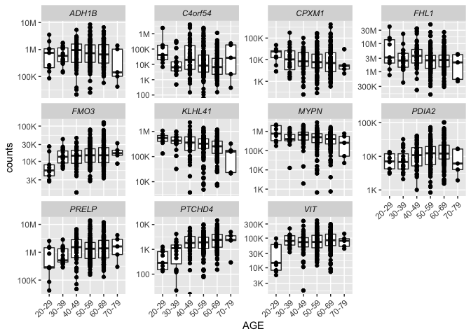
More ggplot()
Now, that we have successfully joined three data frames, we can plot the counts for our differentially expressed genes.
The package scales makes it easy to use scientific notation for the axes. We can also modify the theme() to change the text angle and font face.
library(scales)
## Warning: package 'scales' was built under R version 4.1.2
counts_tidy_long_joined %>%
  ggplot(aes(x = AGE, y = counts)) +
  geom_boxplot() +
  geom_point() +
  facet_wrap(~name, scales = "free_y") +
  theme(axis.text.x = element_text(angle = 45, hjust  = 1),
        strip.text = element_text(face = "italic")) +
  scale_y_log10(labels = label_number_si())
## Warning: `label_number_si()` was deprecated in scales 1.2.0.
## Please use the `scale_cut` argument of `label_number()` instead.
## This warning is displayed once every 8 hours.
## Call `lifecycle::last_lifecycle_warnings()` to see where this warning was generated.

## Warning: Transformation introduced infinite values in continuous y-axis
## Transformation introduced infinite values in continuous y-axis

## Warning: Removed 3 rows containing non-finite values (stat_boxplot).
That completes our section on tidying and transforming data.
Key functions
| Function | Description |
|---|---|
filter() |
A function for filtering data |
mutate() |
A function for create new columns |
select() |
A function for selecting/reordering columns |
arrange() |
A function for ordering observations |
full_join() |
Join 2 tables, return all observations |
left_join() |
Join 2 tables, return all observations in the left and matching observations in the right |
inner_join() |
Join 2 tables, return observations with values in both tables |
pivot_wider() |
Widen a data frame |
pivot_longer() |
Lengthen a data frame |
drop_na() |
Remove missing values |
separate() |
Separate a column into two columns |